Review of Deep Learning Algorithms for Object Detection

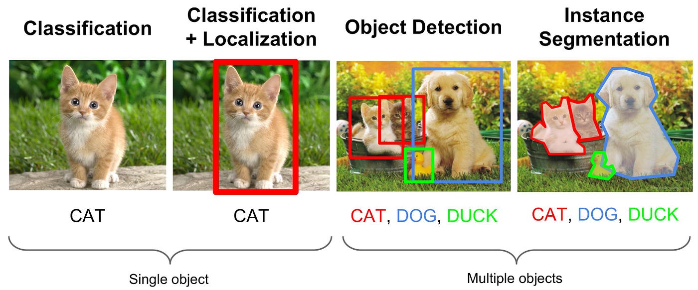
Why object detection instead of image classification?
Image classification models detailed in my previous blog post classify images into a single category, usually corresponding to the most salient object. However at Zyl we are developing features that bring back old memories buried in your smartphone. Photos taken with mobile phones are usually complex and contain multiple objects. This being said, assigning a label with image classification models can become tricky and uncertain. Object detection models are therefore more appropriate to identify multiple relevant objects in a single image. The second significant advantage of object detection models versus image classification ones is that localization of the objects is provided. This wasn’t a relevant criteria for Zyl and features such as photo albums creation or duplicate detection but in other use cases it can be interesting. Think about autonomous cars or caption generation of images.
In this blog post I will review the state-of-the art of object detection models. I will provide details about the evolution of the architectures of the most accurate object detection models from 2012 up to today. One of my analysis criteria will be on their speed at inference allowing real-time analysis. Note that researchers test their algorithms using different datasets (PASCAL VOC, COCO, ImageNet) which are different between the years. Thus the cited accuracies cannot be directly compared per se.
Datasets and Performance Metric
Several datasets have been released for object detection challenges. Researchers publish results of their algorithms applied to these challenges. Specific performance metrics have been developed to take into account the spatial position of the detected object and the accuracy of the predicted categories.
Datasets
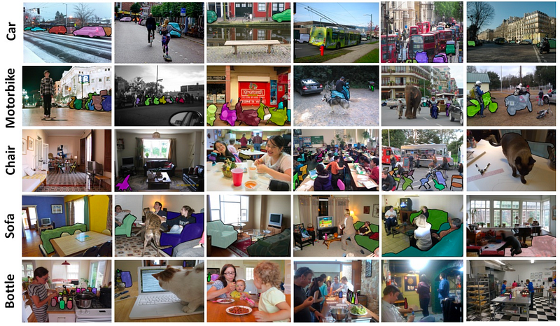
The PASCAL Visual Object Classification (PASCAL VOC) dataset is a well-known dataset for object detection, classification, segmentation of objects and so on. There are 8 different challenges spanning from 2005 to 2012, each of them having its own specificities. There are around 10 000 images for training and validation containing bounding boxes with objects. Although, the PASCAL VOC dataset contains only 20 categories, it is still considered as a reference dataset in the object detection problem.
ImageNet has released an object detection dataset since 2013 with bounding boxes. The training dataset is composed of around 500 000 images only for training and 200 categories. It is rarely used because the size of the dataset requires an important computational power for training. Also, the high number of classes complicates the object recognition task. A comparison between the 2014 ImageNet dataset and the 2012 PASCAL VOC dataset is available here.
On the other hand, the Common Objects in COntext (COCO) dataset is developed by Microsoft and detailed by T.-Y.Lin and al. (2015). This dataset is used for multiple challenges: caption generation, object detection, key point detection and object segmentation. We focus on the COCO object detection challenge consisting in localizing the objects in an image with bounding boxes and categorizing each one of them between 80 categories. The dataset changes each year but usually is composed of more than 120 000 images for training and validation, and more than 40 000 images for testing. The test dataset has been recently cut into the test-dev dataset for researchers and the test-challenge dataset for competitors. Both associated labeled data are not publicly available to avoid overfitting on the test dataset.
Performance Metric
The object detection challenge is, at the same time, a regression and a classification task. First of all, to assess the spatial precision we need to remove the boxes with low confidence (usually, the model outputs many more boxes than actual objects). Then, we use the Intersection over Union (IoU)area, a value between 0 and 1. It corresponds to the overlapping area between the predicted box and the ground-truth box. The higher the IoU, the better the predicted location of the box for a given object. Usually, we keep all bounding box candidates with an IoU greater than some threshold.
In binary classification, the Average Precision (AP) metric is a summary of the precision-recall curve, details are provided here. The commonly used metric used for object detection challenges is called the mean Average Precision (mAP). It is simply the mean of the Average Precisions computed over all the classes of the challenge. The mAP metric avoids to have extreme specialization in few classes and thus weak performances in others.
The mAP score is usually computed for a fixed IoU but a high number of bounding boxes can increase the number of candidate boxes. The COCO challenge has developed an official metric to avoid an over generation of boxes. It computes a mean of the mAP scores for variable IoU values in order to penalize high number of bounding boxes with wrong classifications.
Region-based Convolutional Network (R-CNN)
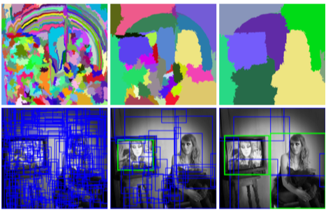
The first models intuitively begin with the region search and then perform the classification. In R-CNN, the selective search method developed by J.R.R. Uijlings and al. (2012) is an alternative to exhaustive search in an image to capture object location. It initializes small regions in an image and merges them with a hierarchical grouping. Thus the final group is a box containing the entire image. The detected regions are merged according to a variety of color spaces and similarity metrics. The output is a few number of region proposals which could contain an object by merging small regions.
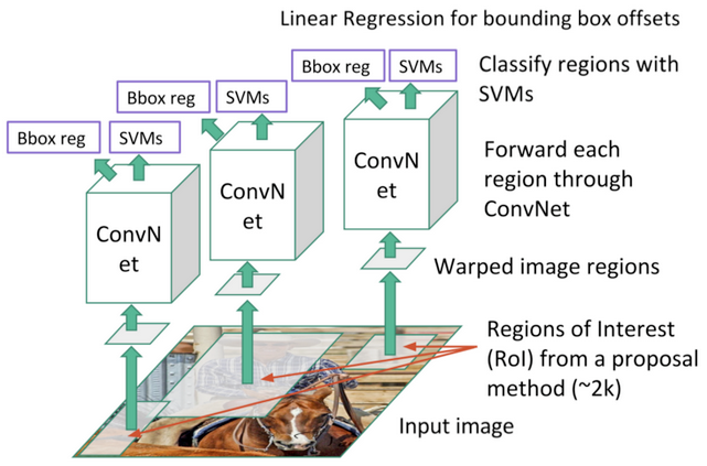
The R-CNN model (R. Girshick et al., 2014) combines the selective searchmethod to detect region proposals and deep learning to find out the object in these regions. Each region proposal is resized to match the input of a CNN from which we extract a 4096-dimension vector of features. The features vector is fed into multiple classifiers to produce probabilities to belong to each class. Each one of these classes has a SVM classifier trained to infer a probability to detect this object for a given vector of features. This vector also feeds a linear regressor to adapt the shapes of the bounding box for a region proposal and thus reduce localization errors.
The CNN model described by the authors is trained on the 2012 ImageNet dataset of the original challenge of image classification. It is fine-tuned using the region proposals corresponding to an IoU greater than 0.5 with the ground-truth boxes. Two versions are produced, one version is using the 2012 PASCAL VOC dataset and the other the 2013 ImageNet dataset with bounding boxes. The SVM classifiers are also trained for each class of each dataset.
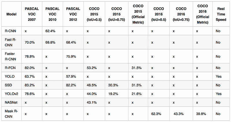
The best R-CNNs models have achieved a 62.4% mAP score over the PASCAL VOC 2012 test dataset (22.0 points increase w.r.t. the second best result on the leader board) and a 31.4% mAP score over the 2013 ImageNet dataset (7.1 points increase w.r.t. the second best result on the leader board).
Fast Region-based Convolutional Network (Fast R-CNN)
The purpose of the Fast Region-based Convolutional Network (Fast R-CNN) developed by R. Girshick (2015) is to reduce the time consumption related to the high number of models necessary to analyse all region proposals.
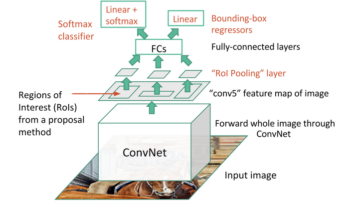
A main CNN with multiple convolutional layers is taking the entire image as input instead of using a CNN for each region proposals (R-CNN). Region of Interests (RoIs) are detected with the selective search method applied on the produced feature maps. Formally, the feature maps size is reduced using a RoI pooling layer to get valid Region of Interests with fixed heigh and width as hyperparameters. Each RoI layer feeds fully-connected layers¹ creating a features vector. The vector is used to predict the observed object with a softmax classifier and to adapt bounding box localizations with a linear regressor.
The best Fast R-CNNs have reached mAp scores of 70.0% for the 2007 PASCAL VOC test dataset, 68.8% for the 2010 PASCAL VOC test dataset and 68.4% for the 2012 PASCAL VOC test dataset.
Faster Region-based Convolutional Network (Faster R-CNN)
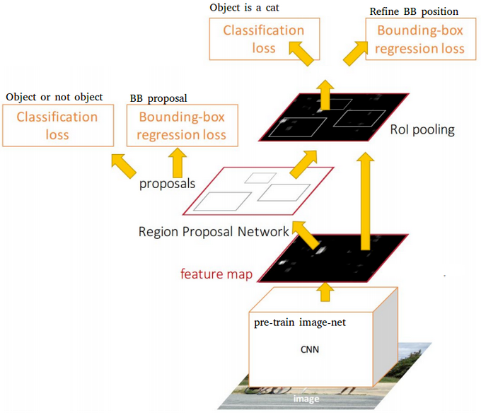
Region proposals detected with the selective search method were still necessary in the previous model, which is computationally expensive. S. Ren and al. (2016) have introduced Region Proposal Network (RPN) to directly generate region proposals, predict bounding boxes and detect objects. The Faster Region-based Convolutional Network (Faster R-CNN) is a combination between the RPN and the Fast R-CNN model.
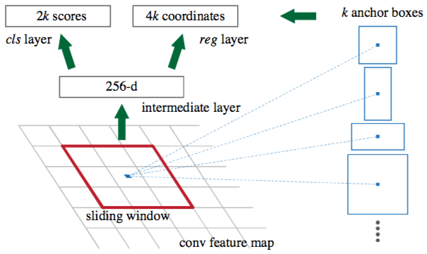
A CNN model takes as input the entire image and produces feature maps. A window of size 3x3 slides all the feature maps and outputs a features vector linked to two fully-connected layers, one for box-regression and one for box-classification. Multiple region proposals are predicted by the fully-connected layers. A maximum of k regions is fixed thus the output of the box-regression layer has a size of 4k (coordinates of the boxes, their height and width) and the output of the box-classification layer a size of 2k (“objectness” scores to detect an object or not in the box). The k region proposals detected by the sliding window are called anchors.
When the anchor boxes are detected, they are selected by applying a threshold over the “objectness” score to keep only the relevant boxes. These anchor boxes and the feature maps computed by the initial CNN model feeds a Fast R-CNN model.
Faster R-CNN uses RPN to avoid the selective search method, it accelerates the training and testing processes, and improve the performances. The RPN uses a pre-trained model over the ImageNet dataset for classification and it is fine-tuned on the PASCAL VOC dataset. Then the generated region proposals with anchor boxes are used to train the Fast R-CNN. This process is iterative.
The best Faster R-CNNs have obtained mAP scores of 78.8% over the 2007 PASCAL VOC test dataset and 75.9% over the 2012 PASCAL VOC test dataset. They have been trained with PASCAL VOC and COCO datasets. One of these models² is 34 times faster than the Fast R-CNN using the selective search method.
Region-based Fully Convolutional Network (R-FCN)
Fast and Faster R-CNN methodologies consist in detecting region proposals and recognize an object in each region. The Region-based Fully Convolutional Network (R-FCN) released by J. Dai and al. (2016) is a model with only convolutional layers³ allowing complete backpropagation for training and inference. The authors have merged the two basic steps in a single model to take into account simultaneously the object detection (location invariant) and its position (location variant).
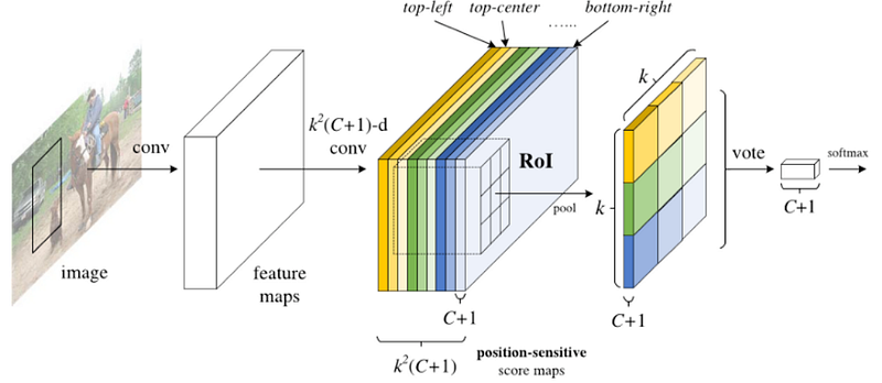
A ResNet-101 model takes the initial image as input. The last layer outputs feature maps, each one is specialized in the detection of a category at some location. For example, one feature map is specialized in the detection of a cat, another one in a banana and so on. Such feature maps are called position-sensitive score maps because they take into account the spatial localization of a particular object. It consists of
k*k*(C+1) score maps where k is the size of the score map, and C the number of classes. All these maps form the score bank. Basically, we create patches that can recognize part of an object. For example, for k=3, we can recognize 3x3 parts of an object.
In parallel, we need to run a RPN to generate Region of Interest (RoI). Finally, we cut each RoI in bins and we check them against the score bank. If enough of these parts are activated, then the patch vote ‘yes’, I recognized the object.
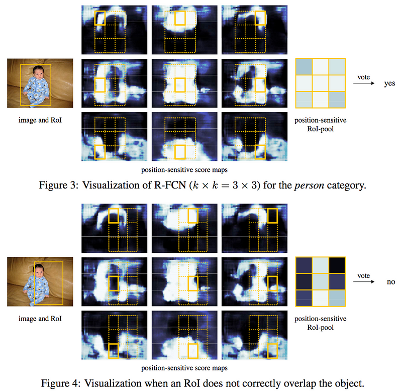
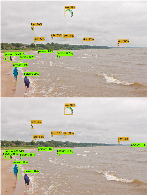
J. Dai and al. (2016) have detailed an example displayed below. The figures show the reaction of a R-FCN model specialized in detecting a person. For a RoI in the center of the image (Figure 3), the subregions in the feature maps are specific to the patterns associated to a person. Thus they vote for ‘yes, there is a person at this location’. In the Figure 4, the RoI is shifted to the right and it is no longer centred on the person. The subregions in the feature maps do not agree on the person detection, thus they vote ‘no, there is no person at this location’.
The best R-FCNs have reached mAP scores of 83.6% for the 2007 PASCAL VOC test dataset and 82.0%, they have been trained with the 2007, 2012 PASCAL VOC datasets and the COCO dataset. Over the test-dev dataset of the 2015 COCO challenge, they have had a score of 53.2% for an IoU = 0.5 and a score of 31.5% for the official mAP metric. The authors noticed that the R-FCN is 2.5–20 times faster than the Faster R-CNN counterpart.
You Only Look Once (YOLO)
The YOLO model (J. Redmon et al., 2016)) directly predicts bounding boxes and class probabilities with a single network in a single evaluation. The simplicity of the YOLO model allows real-time predictions.
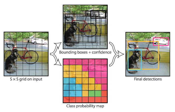
Initially, the model takes an image as input. It divides it into an SxS grid. Each cell of this grid predicts B bounding boxes with a confidence score. This confidence is simply the probability to detect the object multiply by the IoU between the predicted and the ground truth boxes.
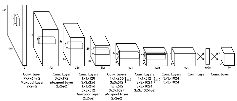
The CNN used is inspired by the GoogLeNet model introducing the inception modules. The network has 24 convolutional layers followed by 2 fully-connected layers. Reduction layers with 1x1 filters⁴ followed by 3x3 convolutional layers replace the initial inception modules. The Fast YOLO model is a lighter version with only 9 convolutional layers and fewer number of filters. Most of the convolutional layers are pretrained using the ImageNet dataset with classification. Four convolutional layers followed by two fully-connected layers are added to the previous network and it is entirely retrained with the 2007 and 2012 PASCAL VOC datasets.
The final layer outputs a
S*S*(C+B*5) tensor corresponding to the predictions for each cell of the grid. C is the number of estimated probabilities for each class. B is the fixed number of anchor boxes per cell, each of these boxes being related to 4 coordinates (coordinates of the center of the box, width and height) and a confidence value.
With the previous models, the predicted bounding boxes often contained an object. The YOLO model however predicts a high number of bounding boxes. Thus there are a lot of bounding boxes without any object. The Non-Maximum Suppression (NMS) method is applied at the end of the network. It consists in merging highly-overlapping bounding boxes of a same object into a single one. The authors noticed that there are still few false positive detected.
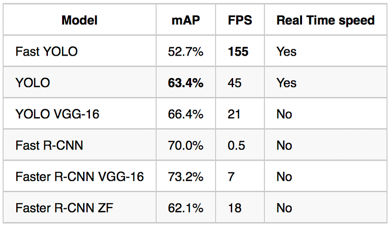
The YOLO model has a 63.7% mAP score over the 2007 PASCAL VOC dataset and a 57.9% mAP score over the 2012 PASCAL VOC dataset. The Fast YOLO model has lower scores but they have both real time performances.
Single-Shot Detector (SSD)
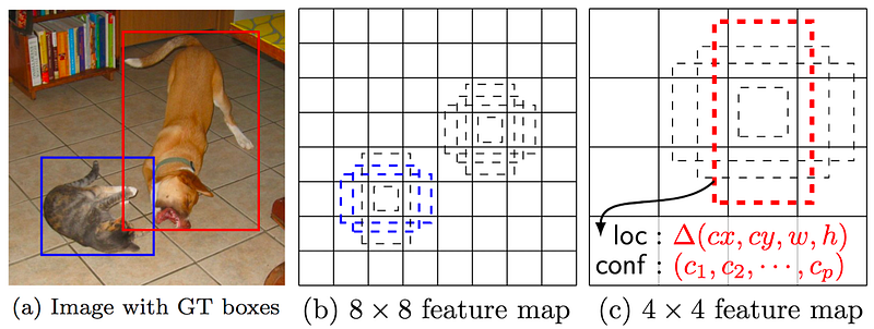
Similarly to the YOLO model, W. Liu et al. (2016) have developed a Single-Shot Detector (SSD) to predict all at once the bounding boxes and the class probabilities with a end-to-end CNN architecture.
The model takes an image as input which passes through multiple convolutional layers with different sizes of filter (10x10, 5x5 and 3x3). Feature maps from convolutional layers at different position of the network are used to predict the bounding boxes. They are processed by a specific convolutional layers with 3x3 filters called extra feature layers to produce a set of bounding boxes similar to the anchor boxes of the Fast R-CNN.
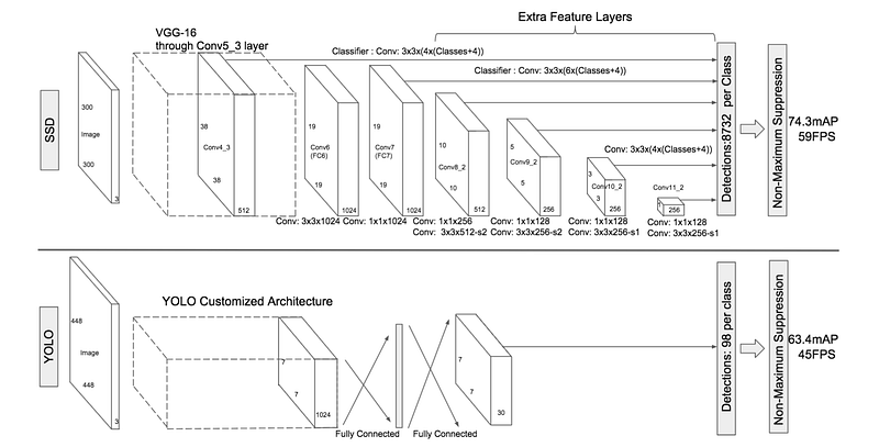
Each box has 4 parameters: the coordinates of the center, the width and the height. At the same time, it produces a vector of probabilities corresponding to the confidence over each class of object.
The Non-Maximum Suppression method is also used at the end of the SSD model to keep the most relevant bounding boxes. The Hard Negative Mining(HNM) is then used because a lot of negative boxes are still predicted. It consists in selecting only a subpart of these boxes during the training. The boxes are ordered by confidence and the top is selected depending on the ratio between the negative and the positive which is at most 1/3.
W. Liu et al. (2016) distinguish the SSD300 model (the architecture is detailed on the figure above) and the SSD512 model which is the SSD300 with an extra convolutional layer for prediction to improve performances. The best SSDs models are trained with the 2007, 2012 PASCAL VOC datasets and the 2015 COCO dataset with data augmentation. They have obtained mAP scores of 83.2% over the 2007 PASCAL VOC test dataset and 82.2% over the 2012 PASCAL VOC test dataset. Over the test-dev dataset of the 2015 COCO challenge, they have had a score of 48.5% for an IoU = 0.5, 30.3% for an IoU = 0.75 and 31.5% for the official mAP metric.
YOLO9000 and YOLOv2
J. Redmon and A. Farhadi (2016) have released a new model called YOLO9000 capable of detecting more than 9000 object categories while running in almost real time according to the authors. They also provide improvements over the initial YOLO model to improve its performances without decreasing its speed (around 10 images per second on a recent mobile according to our implementation).
YOLOv2
The YOLOv2 model is focused on improving accuracy while still being a fast detector. Batch normalization is added to prevent overfitting without using dropout. Higher resolution images are accepted as input: the YOLO model uses 448x448 images while the YOLOv2 uses 608x608 images, thus enabling the detection of potentially smaller objects.
The final fully-connected layer of the YOLO model predicting the coordinates of the bounding boxes has been removed to use anchor boxes in the same way as Faster R-CNN. The input image is reduced to a grid of cells, each one containing 5 anchor boxes. YOLOv2 uses
19*19*5=1805 anchor boxes by image instead of 98 boxes for the YOLO model. YOLOv2 predicts correction of the anchor box relative to the location of the grid cell (the range is between 0 and 1) and selects the boxes according to their confidence as the SSD model. The dimensions of the anchor boxes has been fixed using k-means on the training set of bounding boxes.
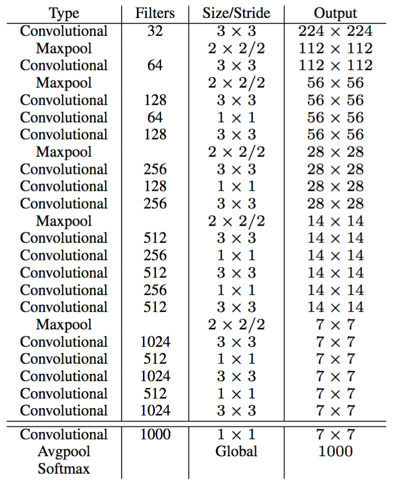
It uses a ResNet-like architecture to stack high and low resolution feature maps to detect smaller objects. The “Darknet-19” is composed of 19 convolutional layers with 3x3 and 1x1 filters, groups of convolutional layers are followed by maxpooling layers to reduce the output dimension. A final 1x1 convolutional layer outputs 5 boxes per cell of the grid with 5 coordinates and 20 probabilities each (the 20 classes of the PASCAL VOC dataset).
The YOLOv2 model trained with the 2007 and 2012 PASCAL VOC dataset has a 78.6% mAP score over the 2007 PASCAL VOC test dataset with a FPS value of 40. The model trained with the 2015 COCO dataset have mAP scores over the test-dev dataset of 44.0% for an IoU = 0.5, 19.2% for an IoU = 0.75 and 21.6% for the official mAP metric.
YOLO9000
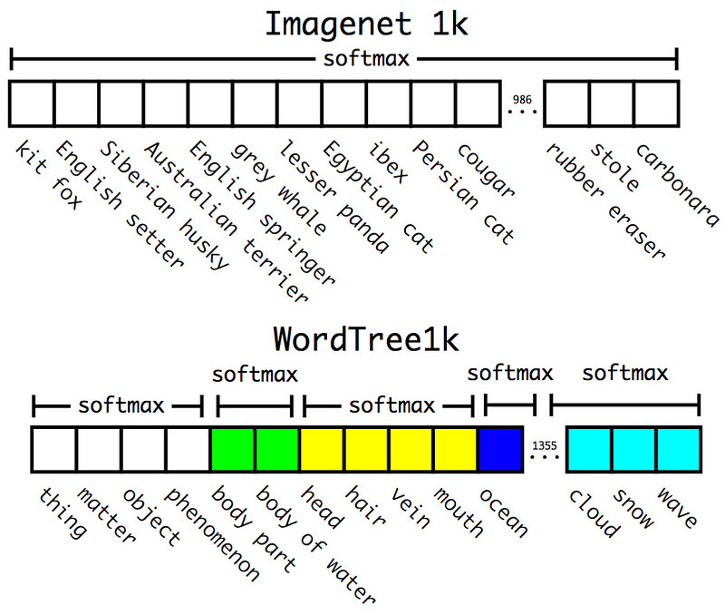
The authors have combined the ImageNet dataset with the COCO dataset in order to have a model capable of detecting precise objects or animal breed. The ImageNet dataset for classification contains 1000 categories and the 2015 COCO dataset only 80 categories. The ImageNet classes are based on the WordNet lexicon developed by the Princeton University⁵ which is composed of more than 20 000 words. J. Redmon and A. Farhadi (2016) detail a method to construct a tree version of the WordNet. A softmax is applied on a group of labels with the same hyponym when the model predicts on an image. Thus the final probability associated to a label is computed with posterior probabilities in the tree. When the authors extend the concept to the entire WordNet lexicon excluding under-represented categories, they obtain more than 9 000 categories.
A combination between the COCO and the ImageNet datasets is used to train a YOLOv2-like architecture with 3 prior convolution layers instead of 5 to limit the output size. The model is evaluated on the ImageNet dataset for the detection task with around 200 labels. Only 44 labels are shared between the training and the testing dataset so the results are somewhat irrelevant. It gets a 19.7% mAP score overall the test dataset.
Neural Architecture Search Net (NASNet)
The Neural Architecture Search (B. Zoph and Q.V. Le, 2017) is detailed in my previous post. It consists in learning the architecture of a model to optimize the number of layers while improving the accuracy over a given dataset. B. Zoph et al. (2017) have reached higher performances with lighter model than previous works over the 2012 ImageNet classification challenge.
The authors have applied this method to spatial object detection. The NASNet network has an architecture learned from the CIFAR-10 dataset and is trained with the 2012 ImageNet dataset. This model is used for feature maps generation and is stacked into the Faster R-CNN pipeline. Then the entire pipeline is retrained with the COCO dataset.
The best NASNet models for object recognition have obtained a 43.1% mAP score over the test-dev dataset of the COCO challenge with an IoU = 0.5. The lighter version of the NASNet optimized for mobile have a 29.6% mAP score over the same dataset.
Mask Region-based Convolutional Network (Mask R-CNN)
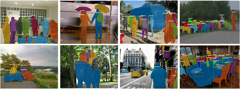
Another extension of the Faster R-CNN model has been released by K. He and al. (2017) adding a parallel branch to the bounding box detection in order to predict object mask. The mask of an object is its segmentation by pixel in an image. This model outperforms the state-of-the-art in the four COCO challenges: the instance segmentation, the bounding box detection, the object detection and the key point detection.
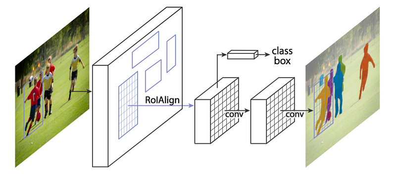
The Mask Region-based Convolutional Network (Mask R-CNN) uses the Faster R-CNN pipeline with three output branches for each candidate object: a class label, a bounding box offset and the object mask. It uses Region Proposal Network (RPN) to generate bounding box proposals and produces the three outputs at the same time for each Region of Interest (RoI).
The initial RoIPool layer used in the Faster R-CNN is replaced by a RoIAlignlayer. It removes the quantization of the coordinates of the original RoI and computes the exact values of the locations. The RoIAlign layer provides scale-equivariance and translation-equivariance with the region proposals.
The model takes an image as input and feeds a ResNeXt network with 101 layers. This model looks like a ResNet but each residual block is cut into lighter transformations which are aggregated to add sparsity in the block. The model detects RoIs which are processed using a RoIAlign layer. One branch of the network is linked to a fully-connected layer to compute the coordinates of the bounding boxes and the probabilities associated to the objects. The other branch is linked to two convolutional layers, the last one computes the mask of the detected object.
Three loss functions associated to each task to solve are summed. This sum is minimized and produces great performances because solving the segmentation task improve the localization and thus the classification.
The Mask R-CNN have reached mAP scores of 62.3% for an IoU = 0.5, 43.4% for an IoU = 0.7 and 39.8% for the official metric over the 2016 COCO test-dev dataset.
Conclusion
Through the years, object detection models tend to infer localization and classification all at once to have an entirely differentiable network. Thus it can be trained from head to tail with backpropagation. Moreover, A trade-off between high performance and realtime prediction capability is made between the recent models.
The models presented in this blog post are either accurate or fast for inference. However, they all have complex and heavy architectures. For example, the YOLOv2 model is around 200MB and the best NASNet around 400MB. Reduction of size while keeping the same performances is an active field of research to embed deep learning models into mobile devices.